Usage
To run SkiftiTools, you must have Nifti image format or tab-separated ASCII format data. SkiftiTools is most commonly used with diffusion MRI data.
Examples
A. Processing OpenNeuro DTI data using SkiftiTools v0.1.1
STEP 1
1.1 OpenNeuro Dataset:
Download shell script under Download with a shell script from OpenNeuro [3]
1.2 Extract the download options for 1st three items
cat ds003900-1.1.1.sh | grep fa.nii.gz | head -3 > ds003900-1.1.1_example_for_skiftiTools.sh
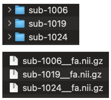
Subjects that are downloaded with only their FA nifti images:
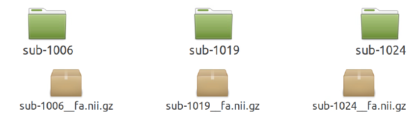
STEP 2
2.1 Run ANTs TBSS on the data.
For this specific example data, use the script tractinferno_prep_ants_tbss.sh and run it in the directory it is downloaded in.
2.2 Then, run the following Docker command, but make sure that you are using memory capacity based on the machine it is running on. ANTs registration is very memory-intensive and the antsRegistrationSyNQuick.sh process can be force killed. It is safer to use flags with the following parameters, although it might run a little slower because of single-threaded processing: --cpus="1" --memory="4g" --ncpu 1
docker run -it --cpus="1" --memory="4g" -v $(pwd):/root/data -v $(pwd)/out_ants_tbss_enigma_ss:/root/data/out_enigma haanme/ants_tbss:0.4.2 -i /root/data/IMAGELIST_ss_docker.csv -c /root/data/CASELIST.txt --modality FA --enigma --ncpu 1 -o /root/data/out_enigma
Output in the terminal should look like this:
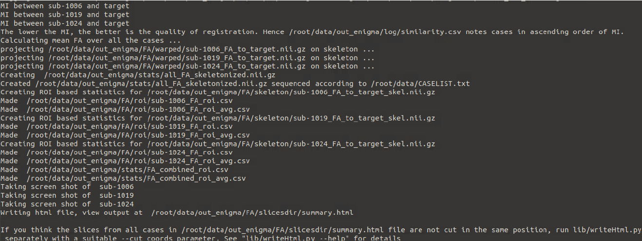
STEP 3
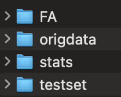
3.1 Check the output created by the ants_tbss Docker. The out_ants_tbss_enigma_ss folder:
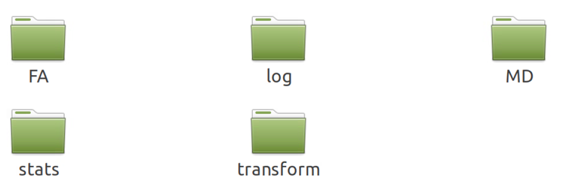
3.2 The most important folder is stats. Open it and make sure that you have the following:
FA_combined_roi_avg.csv
FA_combined_roi.csv
all_FA_skeletonised.nii.gz
mean_FA_skeleton_mask.nii.gz
If any of these files are missing, re-run the Docker, or debug to see what went wrong.
STEP 4
4.1 You can rename the out_ants_tbss_enigma_ss to tbss to keep the directory structure clean.
4.2 Then run the following command in the directory above the tbss folder:
docker run --rm -v $(pwd):/data -it ashjoll/skiftitools:0.1.1 --path /data --outputpath /data/results --TBSSsubfolder tbss --scalar FA --name test
To understand what each flag is doing, you can run:
docker run --rm ashjoll/skiftitools:0.1.1 -h
The skifti data file will be in the results folder, named test_FA_Skiftidata.txt.
Although this file contains only 3 subjects, it can still be difficult to open in Excel/Numbers, etc, due to a lot of data. You can open it in R Studio with the following code:
library(data.table)
skifti <- fread("/path/to/text/file", header = FALSE, skip = 8)
(The first few lines in the text file will have metadata that we don’t need, hence skip = 8).
colnames(skifti) <- c("SubjectID", paste0("V", 1:(ncol(skifti)-1)))
The tabular data should look like this:
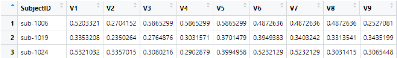
The picture does not display all the columns; there will be many. The V1, V2, V3… are the mean FA in each white matter ROI for each subject.
STEP 5
Perform any kind of complex statistical analysis using this dataset.
B. Processing OpenNeuro DTI data using SkiftiTools v0.2.0
STEP 1
1.1 OpenNeuro Dataset: Download shell script under Download with a shell script from OpenNeuro [3].
1.2 Extract the download options for 1st three items
cat ds003900-1.1.1.sh | grep fa.nii.gz | head -3 > ds003900-1.1.1_example_for_skiftiTools.sh
Subjects that are downloaded with only their FA nifti images:
STEP 2
Run TBSS on the data, can be FSL, ANTS etc.
STEP 3
Check the TBSS output
Make sure to have at least the following files in the stats folder:
/stats/all_FA_skeletonised.nii.gz
/stats/mean_FA_skeleton_mask.nii.gz
STEP 4
Run make_subject_list.sh to create a text file that contains the subject IDs.
STEP 5
Run the docker command:
docker run --rm -v /path/to/tbss/data/:/data ashjoll/skiftitools:0.2.0 --path /data --outputpath /data/results --TBSSsubfolder tbss --subjectsfile /data/subject_list.txt --scalars FA --name test --writemaskcoordinates Yes
To understand what each flag is doing, run:
docker run --rm ashjoll/skiftitools:0.2.0 -h
The Skifti data file will be in the results folder, named test_FA_Skiftidata.txt.
If you used the --writemaskcoordinates, you would find a test_FA_Skiftidata_mask_coordinates.txt folder containing all the coordinates.
Although this test skiftidata file contains only 3 subjects, it can still be difficult to open in Excel/Numbers, etc, due to a lot of voxel data. You can open it in R Studio with the following code:
library(data.table)
skifti <- fread("/path/to/text/file", header = FALSE, skip = 8)
(The first few lines in text file will have metadata that we don’t need, hence skip = 8).
colnames(skifti) <- c("SubjectID", paste0("V", 1:(ncol(skifti)-1)))
The tabular data should look like this:
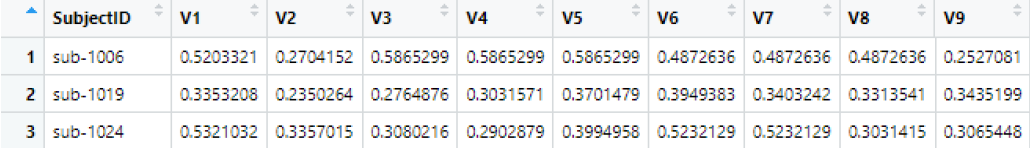
The picture does not display all the columns; there will be many. The V1, V2, V3… are the mean FA in each white matter ROI voxels for each subject.
STEP 6
To integrate the coordinates text file to the skiftidata table in R:
Note
#Coordinates for non-zero voxels
#Load coordinates
coords <- fread("/path/to/test_FA_Skiftidata_mask_coordinates.txt", header = FALSE)
colnames(coords) <- c("X", "Y", "Z")
#Find voxel columns with at least one non-zero value
voxel_cols <- colnames(skifti)[-1]
non_zero_voxels <- voxel_cols[apply(skifti[, ..voxel_cols], 2, function(col) any(col != 0))]
#Subset both data and coordinates
filtered_skifti <- skifti[, c("SubjectID", non_zero_voxels), with = FALSE]
filtered_coords <- coords[match(non_zero_voxels, voxel_cols), ]
#Create new header row with coordinates
coord_labels <- apply(filtered_coords, 1, function(row) paste0("(", row[1], ",", row[2], ",", row[3], ")"))
header_row <- c("Coordinates", coord_labels)
#Combine into final output: add coordinate row as a new row before data
skifti_nonzero <- rbindlist(list(as.list(header_row), filtered_skifti), use.names = FALSE, fill = TRUE)
Output table:

Note
##Coordinates for all voxels##
#Load full coordinates
coords_all <- fread("/path/to/test_FA_Skiftidata_mask_coordinates.txt", header = FALSE)
colnames(coords_all) <- c("X", "Y", "Z")
#Create coordinate labels
coord_labels_all <- apply(coords_all, 1, function(row) paste0("(", row[1], ",", row[2], ",", row[3], ")"))
header_row_all <- c("Coordinates, coord_labels_all)
#Combine coordinate row + subject data
skifti_allvox <- rbindlist(list(as.list(header_row_all), skifti), use.names = FALSE, fill = TRUE)
Output table:

STEP 7
Perform any kind of complex statistical analysis using this tabular data.
References
[3] Philippe Poulin and Guillaume Theaud and Pierre-Marc Jodoin and Maxime Descoteaux (2022). TractoInferno: A large-scale, open-source, multi-site database for machine learning dMRI tractography. OpenNeuro. [Dataset] doi: doi:10.18112/openneuro.ds003900.v1.1.1